Parameter Selection for Temporal Mapper

On this page, we will describe the critical parameters of temporalmapper.TemporalMapper, and give advice on how to select them for your data.

Here’s some test data:

import temporalmapper as tm
import numpy as np
import pandas as pd
import matplotlib.pyplot as plt
import requests, io
from sklearn.cluster import DBSCAN
import datamapplot as dmp

demo_data_file = requests.get("https://github.com/TutteInstitute/temporal-mapper/raw/docs/docs/data/genus1_demo.npy")
X = np.load(io.BytesIO(demo_data_file.content))
X = X[np.argsort(X[:,0])]
fig, ax = plt.subplots(1,1)
ax.scatter(X[:,0],X[:,1],s=0.1,c='k',alpha=0.8)
ax.set_ylabel("Semantic space ($\mathbb{R}^d$)")
ax.set_xlabel("Time")
plt.show()

Number of Time Slices: n_slices

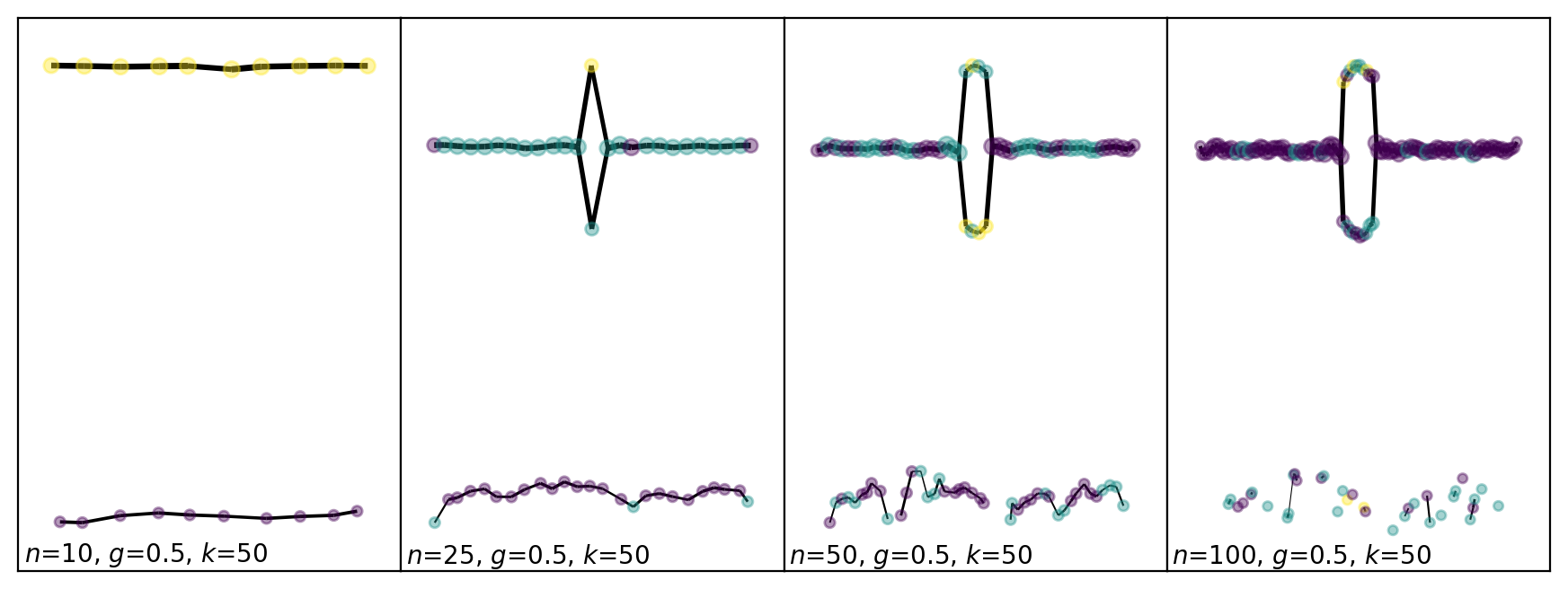
The parameter n_slices has the greatest impact on the output of Mapper, so it is important to make a reasonable choice.

If we had infintely many data points, then the theory tells us that there is some maximum M such that for n_slices > M, the Mapper graph will capture all the topological features. For this reason, we want to take n_slices large. However with finite data, as n_slices is increased, the output graph will become more and more disconnected. This defines the following trade-off:

As n_slices$ :nbsphinx-math:`to`$∞, the amount of features captured increases and the amount of discretization artifacts increases.

To avoid having many artifacts, it is important that each time interval has enough points for the clustering to be reasonable. This gives a heuristic; if you need at least \(s\) points to trust the clustering algorithm, and you have \(n\) samples, then you can take n_slices \(\approxeq n/s\).

For density-based Mapper, which is the default for tm.TemporalMapper, the clustering intervals get strictly larger than in default Mapper (with the same parameters), and hence you can afford to choose a larger n_slices then you would for Mapper.

checkpoint_numbers = [10,25,50,100]

fig, axes = plt.subplots(1,len(checkpoint_numbers))
fig.set_figwidth(11)
fig.set_figheight(4)
fig.dpi = 200
axes = axes.reshape(len(checkpoint_numbers))
clusterer = DBSCAN()
j = 0
for k in range(len(checkpoint_numbers)):
    TM = tm.TemporalMapper(
        clusterer = clusterer,
        n_slices = checkpoint_numbers[k],
        n_neighbors = 100,
        kernel=tm.kernels.square,
    )
    TM.fit(X, time_index=0)
    ax = TM.temporal_plot(ax=axes[k], layout='semantic', cluster_labels={})
    xmin,xmax=axes[k].get_xlim()
    ymin,ymax=axes[k].get_ylim()
    axes[k].text(xmin+0.1,ymin+0.1,fr'$n$={TM.n_slices}, $g$={TM.overlap}, $k$={50}')
    if k%4==3:
        j+=1
plt.subplots_adjust(wspace=0, hspace=0)
plt.show()

Choice of Open Cover: slice_method

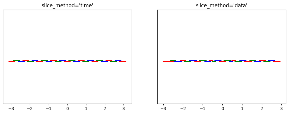
The next most impactful choice is the method used to choose the time-intervals used in Mapper. Temporal Mapper includes two natural choices, slice_method='time' and slice_method='data'. Using time, the intervals are evenly spaced in time, and using data, the intervals have even amounts of data in them. Using time is generally fine, but if your data is very unevenly distributed in time, then using data can provide more consistent results.

Using a sliceograph, we can compare the covers generated by each choice. (Our test data is fairly time-uniform, so the difference is subtle.)

fig, (ax1,ax2) = plt.subplots(1,2,figsize=(12,4))
mapper_time = tm.TemporalMapper(
    clusterer = clusterer,
    n_slices = 25,
    n_neighbors = 100,
    slice_method='time',
    kernel=tm.kernels.square,
)
mapper_time.fit(X, time_index=0)
tm.plotting.view_gomic(mapper_time, ax=ax1)
ax1.set_title("slice_method='time'")

mapper_time = tm.TemporalMapper(
    clusterer = clusterer,
    n_slices = 25,
    n_neighbors = 100,
    slice_method='data',
    kernel=tm.kernels.square,
)
mapper_time.fit(X, time_index=0)
ax2.set_title("slice_method='data'")
tm.plotting.view_gomic(mapper_time, ax=ax2)
plt.show()

Choice of Clustering Algorithm: clusterer

For the most part, your choice of clustering algorithm for Temporal-Mapper is informed by the same trade-offs as any clustering problem. For this purpose, the Scikit-Learn documentation provides a good overview. However, there is one extra thing to note for Temporal Mapper: in Mapper, the clustering algorithm’s purpose is to determine the number of connected components of each slice of the data. Therefore, it is epistemologically backwards to use a clustering algorithm that requires an a-priori choice of number of clusters, such as k-means. Instead, choose something like DBSCAN, which has variable number of clusters.

Number of Nearest-Neighbours: n_neighbors

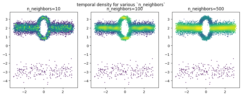
The parameter n_neighbors, or \(k\), is the number of neighbours used in the approximation of the temporal density. As \(k\) and the number of samples grows, the approximation improves. However, for finite sample sizes, increasing \(k\) will average the temporal density as a function of the semantic-space co-ordinates; in the extreme, if \(k>\) n_samples, the temporal density will be constant. Moreover, the \(k\) nearest-neighbours computation is one of the computation bottlenecks in DBMapper, and therefore increasing \(k\) has a noticable performance cost on large datasets.

If your dataset is large (100k+), then we suggest taking \(k\) as large as your computational budget allows. If your dataset is very small, then taking large \(k\) is likely to over-average the temporal density. In this case, start with \(k\) around 50-100.

fig, (ax1,ax2,ax3) = plt.subplots(1,3,figsize=(12,4))
mapper = tm.TemporalMapper(
    clusterer = clusterer,
    n_slices = 25,
    n_neighbors = 10,
    kernel=tm.kernels.square,
)
mapper.fit(X, time_index=0)
ax1.scatter(
    X[:,0],X[:,1],s=1,c=mapper.density
)
ax1.set_title(f"n_neighbors={mapper.n_neighbors}")

mapper = tm.TemporalMapper(
    clusterer = clusterer,
    n_slices = 25,
    n_neighbors = 100,
    kernel=tm.kernels.square,
)
mapper.fit(X, time_index=0)
ax2.set_title(f"n_neighbors={mapper.n_neighbors}")
ax2.scatter(
    X[:,0],X[:,1],s=1,c=mapper.density
)

mapper = tm.TemporalMapper(
    clusterer = clusterer,
    n_slices = 25,
    n_neighbors = 500,
    kernel=tm.kernels.square,
)
mapper.fit(X, time_index=0)
ax3.scatter(
    X[:,0],X[:,1],s=1,c=mapper.density
)
ax3.set_title(f"n_neighbors={mapper.n_neighbors}")
plt.suptitle("temporal density for various `n_neighbors`")
plt.show()

Temporal Kernel: kernel

The choice of temporal kernel has two effects on the output of temporal mapper. The kernel defines weights for the samples, which are passed to the clustering algorithm, and which are used to weigh edges of the output graph.

If you are using a clustering algorithm which does not support sample weights, and you are not using weighted edges on the Mapper graph, then there is no mathematical advantage to using a non-square kernel; in this case set kernel=tm.kernels.square, for a minor performance improvement.

Using the sliceograph plotting function, we can compare the kerneled cover for a square v.s. a a gaussian kernel:

import plotly.io as pio
pio.renderers.default = 'sphinx_gallery'

mapper = tm.TemporalMapper(
    clusterer = clusterer,
    n_slices = 9,
    n_neighbors = 10,
    slice_method='time',
    kernel=tm.kernels.square,
)
mapper.fit(X, time_index=0)
fig = tm.plotting.sliceograph(mapper)
fig.update_layout(title_text="Sliceograph with Square Kernel")
fig.show()

mapper = tm.TemporalMapper(
    clusterer = clusterer,
    n_slices = 9,
    n_neighbors = 10,
    slice_method='data',
    kernel=tm.kernels.gaussian,
)
mapper.fit(X, time_index=0)
fig = tm.plotting.sliceograph(mapper)
fig.update_layout(title_text="Sliceograph with Gaussian Kernel")
fig.show()