Interactive Growth Map
A growth map of a Mapper graph is a visualization that displays each topics relative size and growth. It is inspired by a similar visualization often used to display stock market data.
Let’s demonstrate a growth map by fitting a TemporalMapper to a small dataset of 10,000 arXiv machine learning papers. The paper’s titles and abstracts were concatenated and embedded using the sentence transformer all-mpnet-base-v2, and then reduced to 2D with UMAP.
[1]:
import temporalmapper as tm
import numpy as np
import pandas as pd
import matplotlib.pyplot as plt
import requests, io
from sklearn.cluster import DBSCAN
from fast_hdbscan import HDBSCAN
import datamapplot as dmp
response = requests.get(
    'https://github.com/TutteInstitute/temporal-mapper/raw/refs/heads/docs/docs/data/ai_arxiv_coordinates.npy'
)
map_data = np.load(io.BytesIO(response.content))

response = requests.get(
    'https://github.com/TutteInstitute/temporal-mapper/raw/refs/heads/docs/docs/data/ai_arxiv_data.feather'
)
df = pd.read_feather(io.BytesIO(response.content))

df.head()
[1]:
| title | abstract | id | created | authors | arxiv | doi | |
|---|---|---|---|---|---|---|---|
| 0 | automated rating of recorded classroom present... | effective presentation skills can help to succ... | 1801.00453 | 2018-01-01 | [akzharkyn izbassarova, aidana irmanova, a. p.... | cs.ai | 10.1109/icacci.2017.8125872 |
| 1 | accelerating deep learning with memcomputing | restricted boltzmann machines (rbms) and their... | 1801.00512 | 2018-01-01 | [haik manukian, fabio l. traversa, massimilian... | cs.ai | |
| 2 | accelerating deep learning with memcomputing | restricted boltzmann machines (rbms) and their... | 1801.00512 | 2018-01-01 | [haik manukian, fabio l. traversa, massimilian... | cs.lg | |
| 3 | accurate reconstruction of image stimuli from ... | in neuroscience, all kinds of computation mode... | 1801.00602 | 2018-01-02 | [kai qiao, chi zhang, linyuan wang, bin yan, j... | cs.ai | |
| 4 | deep learning: a critical appraisal | although deep learning has historical roots go... | 1801.00631 | 2018-01-02 | [gary marcus] | cs.lg |
[3]:
# Compute a time column T which is the number of days since Jan 01, 2018.
def date_to_T(date):
    d0 = pd.Timestamp('2018-01-01')
    delta = date-d0
    return delta.days

df["date"] = pd.to_datetime(df["created"])
df["T"] = df["date"].apply(
    lambda x: date_to_T(x)
)
time = df["T"].to_numpy().reshape(-1,1)

clusterer = HDBSCAN(
    cluster_selection_method='eom',
    min_cluster_size=20,
)
mapper = tm.TemporalMapper(
    clusterer = clusterer,
    slice_method = 'data',
    n_slices = 8,
    kernel=tm.kernels.square
)
X = np.concatenate([map_data, time],axis=1)
mapper.fit(X)
[3]:
TemporalMapper(clusterer=HDBSCAN(min_cluster_size=20),
               data=array([[ 4.82239962, -1.57145286],
       [ 1.20892036, -3.84591722],
       [ 1.20193553, -3.85584664],
       ...,
       [11.05540466, 10.08293819],
       [ 8.87438393, -1.76646364],
       [11.04866219, 10.09112167]], shape=(10000, 2)),
               n_slices=8, slice_method='data',
               time=array([  0.,   0.,   0., ..., 480., 480., 480.], shape=(10000,)))
In a Jupyter environment, please rerun this cell to show the HTML representation or trust the notebook. On GitHub, the HTML representation is unable to render, please try loading this page with nbviewer.org.
Parameters
| time | array([ 0., ...hape=(10000,)) | |
| data | array([[ 4.82...pe=(10000, 2)) | |
| clusterer | HDBSCAN(min_cluster_size=20) | |
| n_slices | 8 | |
| n_neighbors | 5 | |
| overlap | 0.5 | |
| inclusion_threshold | 0.01 | |
| slice_method | 'data' | |
| density_based | True | |
| kernel | <function squ...x70ee33ec6a20> | |
| kernel_params | None | |
| verbose | False |
HDBSCAN(min_cluster_size=20)
Parameters
| min_cluster_size | 20 | |
| min_samples | None | |
| cluster_selection_method | 'eom' | |
| allow_single_cluster | False | |
| max_cluster_size | inf | |
| cluster_selection_epsilon | 0.0 | |
| cluster_selection_persistence | 0.0 | |
| semi_supervised | False | |
| ss_algorithm | 'bc' |
Now that we’ve fit a Mapper graph, we can use tm.plotting.growth_map to generate a growth map. The size of each square indicates the number of data points in the corresponding topic, and it’s colour represents the growth of that topic.
[4]:
tm.plotting.growth_map(mapper)
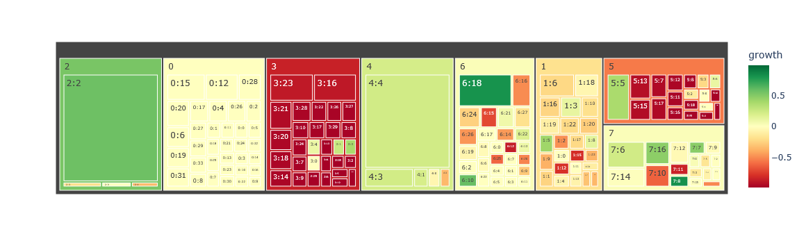
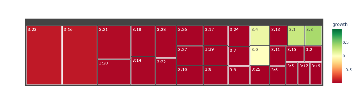
By default, growth_map displays topics across the entire time range, but we can pass an index parameter to show only the topics at a certain time slice.
[6]:
tm.plotting.growth_map(mapper, index=3)
[ ]: